Rafael A. Irizarry's

Music and Statistics Demo

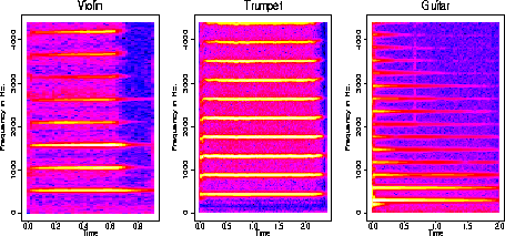
Spectrograms of Harmonic Instruments

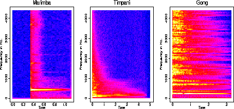
Non-Harmonic Instruments

Low.............................................High

How to play the sounds: This page contains sound examples mentioned in some of my papers related to music and statistics, mainly this one (postscript file). Most sounds, represented by this symbol, are in aiff format which is CD quality. Your audio player should be able to play these files, all you have to do is click. Four of the files are songs so they have been compressed to MP3 files, represented by this symbol . For macs and PCs the RealPlayer (get the FREE version) can play these, for unix you can download . If you want to analyze the music files as data, you should get a program like sox that can convert aiff files to ascii.

Here is a more detailed explanation on how to convert sound signals into ASCII file

Statistical Applications

Statistics has been applied in various ways to music. For example, various stochastic techniques have been applied
in composition. The melody and rhythm in this song

(716 KB mp3 file) are the outcome of a random process. The intervals between each note was produces by a Markov chain. The rhythm was chosen at random from various rhythmic patterns that fit the riffs being played by the bass and the guiro.

Physicist have studied the spectral properties of different musical signals and speculated on the possibility of it being so called 1/f noise (learn more about 1/f noise and music from a paper I wrote with David Brillinger).The following 3 mp3 files are melodies produced with outcomes of an IID process (white noise), a random walk (brown noise) and a process with 1/f noise (pink noise):

White music (236 KB mp3 file).

Brown music (214 KB mp3 file).

Pink music (295 KB mp3 file).

Sound Synthesis and Analysis

The application that most interests me is sound synthesis and analysis. Sound can be represented as a real-valued function of time. This function can be sampled at a small enough rate so that the resulting discrete version is a good approximation of the continuous one. This permits one to study musical sounds as a discrete time series, an entity for which many statistical techniques are available. Physical modeling suggests that many musical instruments' sounds may be characterized by a
deterministic locally periodic and stochastic signal model. In general harmonic instruments are better described by this model than non harmonic ones.

The violin ,trumpet and guitar are all harmonic instruments. The graphs at the beginning of the demo are spectrograms of the sound signals. Notice the yellow lines at multiples of the fundamental frequency we hear. The marimba, timpani and gong are non-harmonic.

It is believed that the strength of at the different multiple frequencies (the harmonics) somehow determine pitch. The trumpet has many strong harmonics which is associated with a bright sound. A clarinet has few strong harmonics. Notice the difference in sound and in their periodograms. The high values in the spectrogram that are not at harmonic frequencies is what we model as a stochastic signal. Notice that the non-harmonic instruments have a lot of "noise".

Separation of signal and noise

We are interested in separating the approximately periodic from the stochastic signal and finding parametric representations with musical meaning. To do so a local harmonic model that tracks changes in pitch and in the amplitudes of the harmonics is fit. We are assuming a model y(t) = s(t) + e(t), with s(t) an approximately periodic function and e(t) noise. The deterministic signal s(t) will have period inversely proportional to the fundamental frequency being played. We estimate s(t) using local harmonic estimation and use the residuals of this fit as the estimate of e(t).

Here are some examples of the separation of the two parts: (all files have been amplified to same volume)

Instrument	Original	Fitted	Residuals
violin
clarinet
guitar
didjiridoo

Notice that the residuals sound very much like what we would expect: a screechy metallic sound for the violin, surplus blown air for the clarinet, and a pluck with no tone for the guitar. Notice how the separation doesn't work very well for the non-harmonic didjiridoo.

Window Size Selection

Deterministic changes in the signal, such as pitch change, suggest that different temporal

window sizes should be considered in the local estimation. Ways to choose appropriate window sizes are developed in this paper (postscript file). We carry out the an estimation for a

shakuhachi flute sound characterized by 3 segment: Rapid change of pitch (0 - 0.5 secs), fix pitch (0.5 - 3.0 secs), tremolo (3.0 - 4.0 secs), and fixed pitch to end the sound. This flute is also characterized by a noisy (windy) sound. We fit our procedure with a fixed small window size, a fixed large window size, and then using an adaptive window size.

Window Size	Fitted	Residual
Fixed Large
Fixed Small
Dynamic choice

If we listen to the sound or look at residual plots we notice that the fixed windows over fit and under fit respectively. In the residuals sound for the large window fit we hear signal during the tremolo and for the small window size fit the fitted signal sounds too noisy, too similar to the original. In this plot we see how the dynamic window chooses smaller size in parts that are less stable.

Applications

Amongst other things our analysis provides estimates of the harmonic signal and of the noise signal. Different musical composition applications may be based on the estimates. The procedure separates harmonic component and noise component of signal, provides pitch estimates, and the harmonic signal is reconstructed into individual harmonics.This plot is an example of the resulting estimates from an oboe sound :

Uses in composition

The function s(t) is defined by parameters that represent local pitch, and local amplitude and phase of the harmonics. We may tweak the estimates of these parameters to modify s(t) and construct a new sound based on the original. We can change pitch, duration, and timbre independently of each other. As an example we run the analysis on an

oboe sound. Musicians say that if one listens to the sound of an oboe closely the sound of a soprano is heard at an octave above the pitch of the oboe sound. By wiggling the estimated amplitudes of the even harmonics we can make the

hidden soprano come out. We can amply the residuals obtained when analyzing the violin to create the sound of a

violin played by a beginner .

Removing Reverberation

When an instrument is played in a room with echo, signals from previous notes may be heard after the instrument has stopped producing the notes. Notice in the sound of a

pipe organ playing two notes how we can hear the first note during the playing of the second. This can clearly be seen in the spectrogram. During the playing of the second note, the yellow line related to the first note is still there. We also see the presence of an approximately periodic component around the 50 Hz. frequency, this is probably due to the sound of the wind going through the organ pipes, an important sounds that helps our ears know it's an organ. If we assume the deterministic signal s(t) is locally periodic with period equal to the fundamental frequency being played and use local harmonic estimation to estimate s(t) and e(t), then the spectrogram of the residuals shows a yellow line representing the reverb note and . Not a good fit. We can also perform residual analysis by ear by listening to the

sound of the residuals. If we listen to the

estimate of s(t), it sounds similar to the original, they are different because we don't hear the reverb during the second note, and also the 50 Hz frequency is not heard. It doesn't really sound like an organ anymore. Now if we instead fit a model with s(t) composed of three periodic components s₁(t), s₂(t), and s₃(t), we obtain a better fit and a separation of each component. We can look at plots showing the results and also listen to them:

Original sound fitted s₁(t) fitted s₂(t)fitted s₃(t)residuals

Note: If you have small speakers with no bass, you probably won't hear some of these sounds.

I couldn't have made this page without the help of David Wessel, Adrian Freed, Matt Wright and the people at CNMAT.

And also Ofer Licht, Phil Spector and David Brillinger from the stat department at Berkeley.

Get the details from this paper.