Compendium for "Seasonal analyses of air pollution and
mortality in 100 U.S. cities" by Peng, et al. (2005)
Abstract
Time series models relating short-term changes in air
pollution levels to daily mortality counts typically assume that
the effects of air pollution on the log relative rate of
mortality do not vary with time. However, these short-term
effects might plausibly vary by season. Changes in the sources of
air pollution and meteorology can result in changes in
characteristics of the air pollution mixture across seasons. The
authors developed Bayesian semiparametric hierarchical models for
estimating time-varying effects of pollution on mortality in
multisite time series studies. The methods were applied to the
database of the National Morbidity and Mortality Air Pollution
Study, which includes data for 100 US cities, for the period
1987--2000. At the national level, a 10-µg/m3
increase in particulate matter less than 10 µm in
aerodynamic diameter at a 1-day lag was associated with 0.15%
(95% posterior interval (PI): -0.08, 0.39), 0.14% (95% PI: -0.14,
0.42), 0.36% (95% PI: 0.11, 0.61), and 0.14% (95% PI: -0.06,
0.34) increases in mortality for winter, spring, summer, and
fall, respectively. An analysis by geographic region found a
strong seasonal pattern in the Northeast (with a peak in summer)
and little seasonal variation in the southern regions of the
country. These results provide useful information for
understanding particle toxicity and guiding future analyses of
particle constituent data.
The
full text of the article is available from the American
Journal of Epidemiology.
Vignette/Compendium
The file seasonal.Rnw is contains
the text for the paper and the R code for creating the figures
and tables. The file can be processed using the Sweave
function in R after running the two "core" analyses below.
To process the vignette, you first need to have a working
LaTeX system and R. R can be downloaded from CRAN.
Save the vignette file in a directory on your computer. You
also need to download the BibTeX
bibliography database to create the final product. After
starting up R:
- Run the core analyses below by executing the code in
core1.R and core2.R. Make sure that the "Other Code and Data"
files are in the "data" sub-directory.
- The core analyses should create a directory "results" where
the results of analyses are cached. In R, run the following:
Sweave("seasonal.Rnw")  ## This will take a few minutes
library(tools)
texi2dvi("seasonal.tex", pdf = TRUE)
This will create a PDF file in the working directory called
"seasonal.pdf".
- To extract the code for the figures and tables, run
library(tools)
Stangle("seasonal.Rnw", split = TRUE)
This will create a separate file for each figure/table
containing the relevant code.
Required R Packages
| NMMAPSdata |
R package containing all of the mortality, air pollution,
and weather data for the National Morbidity, Mortality, and
Air Pollution Study, 1987--2000, 108 U.S. cities. |
| tlnise |
Two-Level Normal Independent Sampler Estimation software
for R (S-PLUS original by Phil Everson) |
| tsModelSpec |
Tools for time series regression model specification |
Packages not listed here that are necessary for reproducing
the results are available from CRAN.
Other Code and Data
The following code files should reside in a subdirectory
called "data".
| model-fitting.R |
Model fitting functions |
| utils.R |
Miscellaneous utility functions for pooling coefficients
and processing results |
| multipollutant.R |
Data processing function for multi-pollutant
database |
| cityList.R |
List of cities used in 100 city analysis analysis (also
including Anchorage, AK and Honolulu, HI) |
| copoll-cityList.R |
List of cities used in 45 city copollutant analysis |
| citynames.csv |
Names of cities used |
Core Data Analysis
The code below creates a sub-directory "results" where
specific results are stored for later use.
Core analysis 1:
- Build database for co-pollutant models
(PM10, ozone, SO2,
NO2)
- Compute smooth seasonally varying effects of
PM10 on non-accidental mortality
- Compute separate seasonal effects of PM10
on non-accidental mortality adjusting for gases
- Compute separate seasonal effects of PM10
on non-accidental mortality (no adjustment for
gases)
|
|
Core analysis 2:
- Compute non-seasonal effects of PM10 on
non-accidental mortality
- Compute smooth seasonally varying effects of
PM10 on non-accidental mortality using
orthogonal sine/cosine basis
- Sensitivity analysis with respect to the degrees of
freedom in the smooth fucnction of time used to adjust
for smooth time varying confounders
|
|
Breakdown of Figures and Tables
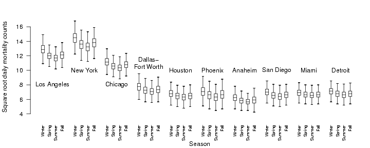
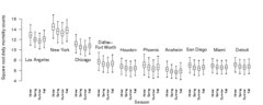 Boxplots of square root daily
mortality by season for the 10 largest U.S. cities,
1987--2000. Boxplots of square root daily
mortality by season for the 10 largest U.S. cities,
1987--2000. |
|
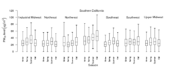 Boxplots of
regionally averaged daily levels of particulate matter less
than 10 $\mu$m in aerodynamic diameter (PM10) by
season for 100 U.S. cities, 1987--2000. Boxplots of
regionally averaged daily levels of particulate matter less
than 10 $\mu$m in aerodynamic diameter (PM10) by
season for 100 U.S. cities, 1987--2000. |
|
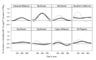
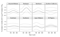 National and
regional smooth seasonal effects of PM10
(particulate matter less than 10 $\mu$m in aerodynamic
diameter) at lag 1 for 100 U.S. cities, 1987--2000. Estimates
were obtained by pooling city-specific coefficients from the
sine/cosine model (equation 2). Dotted lines indicate
pointwise 95 posterior intervals. National and
regional smooth seasonal effects of PM10
(particulate matter less than 10 $\mu$m in aerodynamic
diameter) at lag 1 for 100 U.S. cities, 1987--2000. Estimates
were obtained by pooling city-specific coefficients from the
sine/cosine model (equation 2). Dotted lines indicate
pointwise 95 posterior intervals. |
|
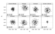 Samples from the
national and regional joint posterior distributions of the
pooled coefficients $\beta_1$ and $\beta_2$ from sine/cosine
seasonal model (equation 2) for PM10 at lag 1, 100
U.S. cities, 1987--2000. The solid and dashed lines indicate
the 75% and 95% regions for the joint posterior distribution
of $\beta_1$ and $\beta_2$, given the data. Each panel
includes the marginal posterior probabilities of each
coefficient being greater than 0. Posterior probabilities
closer to 1 indicate stronger evidence of seasonal
patterns. Samples from the
national and regional joint posterior distributions of the
pooled coefficients $\beta_1$ and $\beta_2$ from sine/cosine
seasonal model (equation 2) for PM10 at lag 1, 100
U.S. cities, 1987--2000. The solid and dashed lines indicate
the 75% and 95% regions for the joint posterior distribution
of $\beta_1$ and $\beta_2$, given the data. Each panel
includes the marginal posterior probabilities of each
coefficient being greater than 0. Posterior probabilities
closer to 1 indicate stronger evidence of seasonal
patterns. |
|
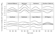
 Sensitivity of
national and regional estimates of smooth seasonal effects
for PM10 at lag 1 to the degrees of freedom
assigned to the smooth function of time, 100 U.S. cities,
1987--2000. The degrees of freedom chosen were 3 (short
dashed), 5 (dotted), 7 (solid), 9 (dot-dashed), and 11 (long
dashed) degrees of freedom per year of data. Sensitivity of
national and regional estimates of smooth seasonal effects
for PM10 at lag 1 to the degrees of freedom
assigned to the smooth function of time, 100 U.S. cities,
1987--2000. The degrees of freedom chosen were 3 (short
dashed), 5 (dotted), 7 (solid), 9 (dot-dashed), and 11 (long
dashed) degrees of freedom per year of data. |
|
 Sensitivity of
national and regional estimates of smooth seasonal effects to
PM10 exposure lag, 100 U.S. cities, 1987--2000.
Solid black lines indicate the log relative rate estimate and
pointwise 95% posterior intervals for PM10 at lag
1. Also shown are the log relative rate estimates for
PM10 at lag 0 (short dashed) and lag 2
(dot-dashed). Sensitivity of
national and regional estimates of smooth seasonal effects to
PM10 exposure lag, 100 U.S. cities, 1987--2000.
Solid black lines indicate the log relative rate estimate and
pointwise 95% posterior intervals for PM10 at lag
1. Also shown are the log relative rate estimates for
PM10 at lag 0 (short dashed) and lag 2
(dot-dashed). |
|
| Table 2: National average estimates of the overall and
season-specific effects of PM10 at lags of 0, 1,
and 2 days for 100 US cities, National Morbidity and
Mortality Air Pollution Study, 1987--2000 |
|
| Table 3: National average estimates of season-specific
lag 1 PM10 log relative rates adjusted for other
pollutants, National Morbidity and Mortality Air Pollution
Study, 1987--2000 |
|
 Boxplots of square root daily
mortality by season for the 10 largest U.S. cities,
1987--2000.
Boxplots of square root daily
mortality by season for the 10 largest U.S. cities,
1987--2000.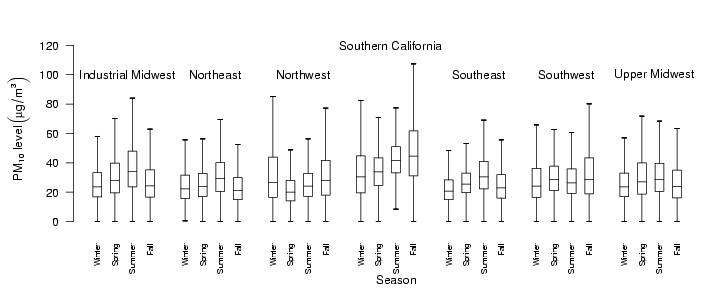 Boxplots of
regionally averaged daily levels of particulate matter less
than 10 $\mu$m in aerodynamic diameter (PM10) by
season for 100 U.S. cities, 1987--2000.
Boxplots of
regionally averaged daily levels of particulate matter less
than 10 $\mu$m in aerodynamic diameter (PM10) by
season for 100 U.S. cities, 1987--2000.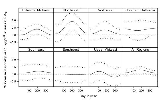 National and
regional smooth seasonal effects of PM10
(particulate matter less than 10 $\mu$m in aerodynamic
diameter) at lag 1 for 100 U.S. cities, 1987--2000. Estimates
were obtained by pooling city-specific coefficients from the
sine/cosine model (equation 2). Dotted lines indicate
pointwise 95 posterior intervals.
National and
regional smooth seasonal effects of PM10
(particulate matter less than 10 $\mu$m in aerodynamic
diameter) at lag 1 for 100 U.S. cities, 1987--2000. Estimates
were obtained by pooling city-specific coefficients from the
sine/cosine model (equation 2). Dotted lines indicate
pointwise 95 posterior intervals. Samples from the
national and regional joint posterior distributions of the
pooled coefficients $\beta_1$ and $\beta_2$ from sine/cosine
seasonal model (equation 2) for PM10 at lag 1, 100
U.S. cities, 1987--2000. The solid and dashed lines indicate
the 75% and 95% regions for the joint posterior distribution
of $\beta_1$ and $\beta_2$, given the data. Each panel
includes the marginal posterior probabilities of each
coefficient being greater than 0. Posterior probabilities
closer to 1 indicate stronger evidence of seasonal
patterns.
Samples from the
national and regional joint posterior distributions of the
pooled coefficients $\beta_1$ and $\beta_2$ from sine/cosine
seasonal model (equation 2) for PM10 at lag 1, 100
U.S. cities, 1987--2000. The solid and dashed lines indicate
the 75% and 95% regions for the joint posterior distribution
of $\beta_1$ and $\beta_2$, given the data. Each panel
includes the marginal posterior probabilities of each
coefficient being greater than 0. Posterior probabilities
closer to 1 indicate stronger evidence of seasonal
patterns. Sensitivity of
national and regional estimates of smooth seasonal effects
for PM10 at lag 1 to the degrees of freedom
assigned to the smooth function of time, 100 U.S. cities,
1987--2000. The degrees of freedom chosen were 3 (short
dashed), 5 (dotted), 7 (solid), 9 (dot-dashed), and 11 (long
dashed) degrees of freedom per year of data.
Sensitivity of
national and regional estimates of smooth seasonal effects
for PM10 at lag 1 to the degrees of freedom
assigned to the smooth function of time, 100 U.S. cities,
1987--2000. The degrees of freedom chosen were 3 (short
dashed), 5 (dotted), 7 (solid), 9 (dot-dashed), and 11 (long
dashed) degrees of freedom per year of data. Sensitivity of
national and regional estimates of smooth seasonal effects to
PM10 exposure lag, 100 U.S. cities, 1987--2000.
Solid black lines indicate the log relative rate estimate and
pointwise 95% posterior intervals for PM10 at lag
1. Also shown are the log relative rate estimates for
PM10 at lag 0 (short dashed) and lag 2
(dot-dashed).
Sensitivity of
national and regional estimates of smooth seasonal effects to
PM10 exposure lag, 100 U.S. cities, 1987--2000.
Solid black lines indicate the log relative rate estimate and
pointwise 95% posterior intervals for PM10 at lag
1. Also shown are the log relative rate estimates for
PM10 at lag 0 (short dashed) and lag 2
(dot-dashed).