by Ann Lehman and John Sall
SAS Institute Inc.
Regression is a method of fitting curves through data points. So why is it called regression?
Sir Francis Galton, in his 1885 Presidential address before the anthropology section of the British Association for the Advancement of Science (Stigler, 1986), described a study he had made that compared the heights of children with the heights of their parents. He examined the heights of parents and their grown children, perhaps to gain some insight into what degree height is an inherited characteristic. He published his results in a paper, "Regression Towards Mediocrity In Hereditary Stature," (Galton, F. (1886)).
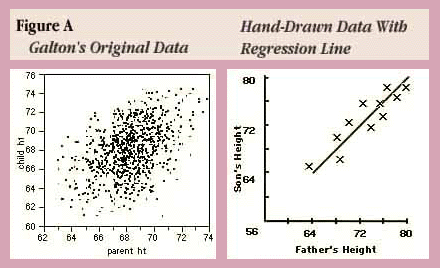
Figure A shows a JMP scatterplot of Galton's original data. The right-hand plot is his attempt to summarize the data and fit a line. He multiplied the womens' heights by 1.08 to make them comparable to mens' heights and defined the parent's height as the average of the two parents. He defined ranges of parents' heights and calculated the mean child's height for each range. Then he drew a straight line that went through the means as best he could.
He thought he had made a discovery when he found that the heights of the children tended to be more moderate than the heights of their parents. For example, if parents were very tall the children tended to be tall but shorter than their parents. If parents were very short the children tended to be short but taller than their parents were. This discovery he called "regression to the mean," with the word "regression" meaning to come back to.
However, Galton's original regression concept considered the variance of both variables, as does orthogonal regression, which is discussed later. Unfortunately, the word "regression" later became synonomous with the least squares method, which assumes the X values are fixed.
To investigate Galton's situation you can look at the Galton.jmp data table, found in the JMP-IN sample library. Use the Fit Y by X command in the Analyze menu with child ht as Y and parent ht as X. Select Fit Line from the Fitting popup menu to see a least squares regression line.
Galton's regression fitted an arbitrary line and then tested to see if the slope of the line was 1. If the line has a slope of 1, then the predicted height of the child is the same as that of the parent, except for a generational constant. A slope of less than one indicates regression in the sense that the children tended to have more moderate heights (closer to the mean) than the parents. Indeed, the left plot in Figure B shows that the least squares regression slope is .61, far below 1, which confirms the regression toward the mean.
But if the heights of the children were more moderate than the heights of the parents, shouldn't the parents' heights be more extreme than the children's?
To find out, you can reverse the model and try to predict the parents' heights from the children's heights. The analysis on the right in Figure B shows the results when parent ht is Y and child ht is X. If there was symmetry this analysis would give a slope greater than 1 because the previous slope was less than one. Instead it is .29, even less than the first slope.
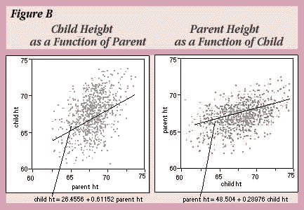
When you do least squares regression there is no symmetry between the Y and X variables. The slope of Y on X is not the reciprocal of the slope of X on Y; you cannot solve the X by Y fit by taking the Y by X fit and solving for the other variable.
The reason there is no symmetry is that the error is minimized in one direction only—that of the Y variable. So if you switch the roles, you are solving a different problem.
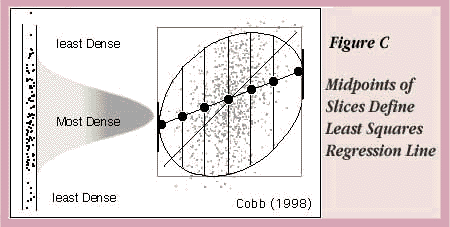
An interesting way to visualize regression is to draw a bivariate density ellipse on a scatterplot. The shape and orientation of an ellipse can quickly characterize the relationship of two variables. In fact, Cobb (1998) talks about regression and correlation as balloon summaries.
He also uses the density ellipse to graphically illustrate the least squares regression line. On the left in Figure C you see a slice of normally distributed points from a scatterplot. For a given range of X values, a reasonable prediction is the Y value in the vertical slice where the points are the densest—the value under the peak of the normal curve. In fact, this is the least squares prediction. The ellipse in Figure C has slices marked at their midpoints. The line through the midpoints of the slices intersects the vertical tangents of the ellipse and is the least squares regression line.
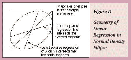
Note that the major axis of the ellipse, which might intuitively seem like it ought to be the regression line, does not cut the midpoints of the slices. For standardized data with X and Y scaled the same, the line along this axis is familiar—it's called the first principal component.
However, there is a way to fit a slope symmetrically, so that the role of both variables is the same. It is called orthogonal regression, and uses the ratio of measurement error (error in the X variable) to the response error (error in the Y variable) in equations to estimate intercept and slope parameters (Fuller, 1987). This ratio,
s2X/s2Y
is zero in the standard least squares regression situation where the variation in X is ignored or assumed be zero, and becomes infinitely large when the variation of Y approaches zero. An interesting advantage to this approach is that the computations give you predicted values for both Y and X.
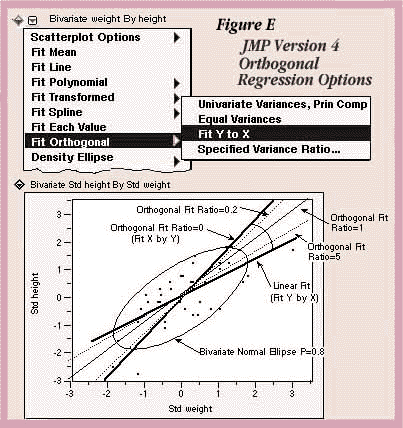
Orthogonal Regression is a new fitting option on the Fit Y by X platform and will be available in JMP Version 4 with the following options (see Figure E) to specify a variance ratio:
The scatterplot in Figure E shows standardized height and weight values with various line fits that illustrate the behavior of the orthogonal line selections. The standard linear regression occurs when the variance of the X variable is considered to be zero. Fit X by Y is the opposite extreme, when the variation of the Y variable is ignored.
All other lines fall between these two extremes and shift as the variance ratio changes. As the variance ratio increases, the variation in the Y response dominates and the slope of the fitted line shifts closer to the Y by X fit. Likewise, when you decrease the ratio, the slope of the line shifts closer to the X by Y fit.
A biographical note: Galton was the cousin of Darwin and mentor of Karl Pearson. This British statistician was also an explorer, and anthropologist, and perfected an early technique for fingerprinting. (The first legal use of fingerprints was in the conviction of a billiard ball thief in 1902.)
References
Cobb, G.W. (1998), Introduction to Design and Analysis of
Experiments, Springer-Verlag: New York.
Galton, F. (1886), "Regression
Towards Mediocrity in Hereditary Stature," Journal of the Anthropological
Institute, 246-263.
Fuller, W. A. (18987), Measurement Error Models, John
Wiley & Sons, New York,
Stigler, S.M. (1986), The History of Statistics,
Cambridge: Belknap Press of Harvard Press.