Sample Code & Output

blue, R output is in black, my comments and explanations are in green.

#First we need to load the Package and the Demo data set
library(CompModel)

data(demo.counts)

# Next we get a quick idea of the Column names in the data and the structure of the Demo data object
names(demo.counts)
[1] "strain"         "exp"            "time"           "field"        
[5] "remained.field" "attached"       "penetrating"    "invaded"      

str(demo.counts)
`data.frame':    189 obs. of  8 variables:
 $ strain        : chr  "demo_strain" "demo_strain" "demo_strain" "demo_strain" ...
 $ exp           : int  1 1 1 1 1 1 1 1 1 1 ...
 $ time          : num  0 0 0 0 0 0 0 0 0 0.5 ...
 $ field         : int  1 2 3 4 5 6 7 8 9 1 ...
 $ remained.field: int  1381 1381 1381 1381 1381 1381 1381 1381 1381 1381 ...
 $ attached      : int  2 7 9 8 2 4 4 2 1 41 ...
 $ penetrating   : int  0 1 0 0 2 0 1 0 0 2 ...
 $ invaded       : int  0 0 0 0 0 0 0 0 0 4 ...

# We will store our work in the object "Demo"
Demo<-NULL

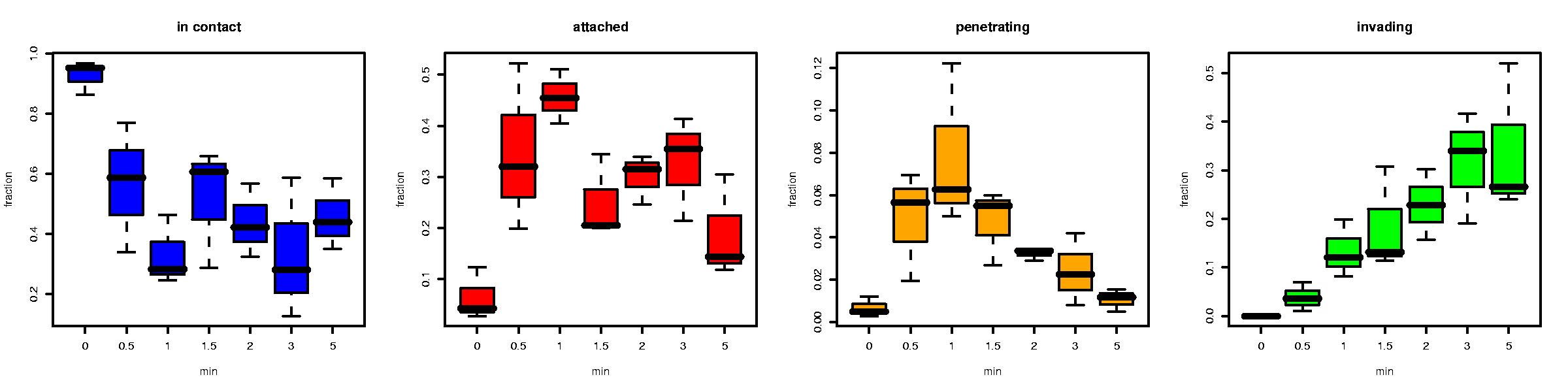
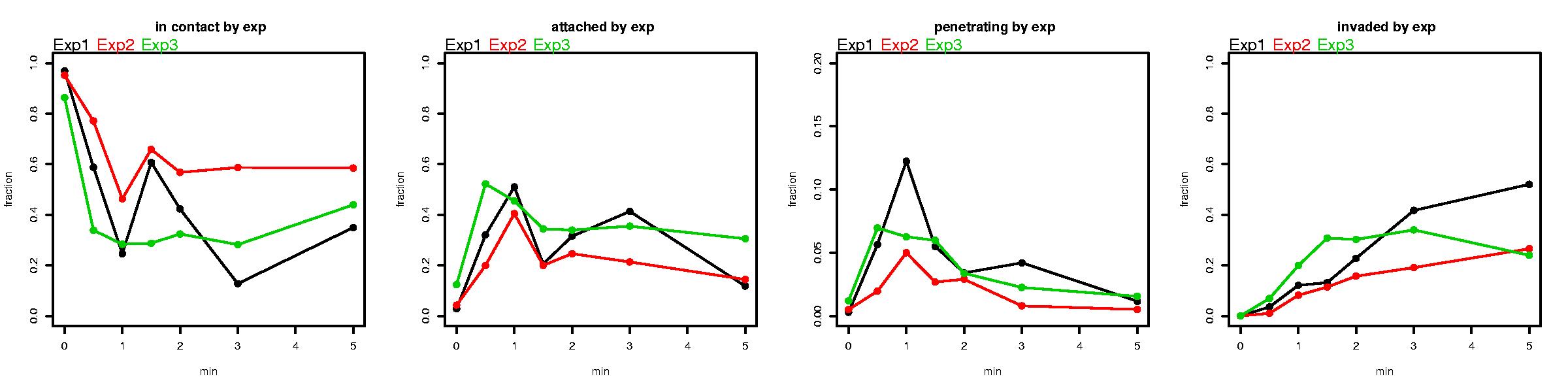
# Now we use the SumFields() function to transform the demo.counts data into a form that we can use for modeling. We also use the PlotByTime() and PlotByExp() functions to get an idea of what the data looks like and look for anything extraordinary

Demo$sum<-SumFields(demo.counts)

PlotByTime(Demo$sum)


PlotByExp(Demo$sum) 


# Define the model including intial paramters guess ($parms), the times to evaluate ($times), the initial conditions of the system ($init), the residual weights ($weights), the ODEs ($form) and the log-transformed ODEs ($logform)

Model<-NULL
Model$parms<-c("k1"=1.0,"k2"=1.0,"k3"=0.5,"k4"=3.0)
Model$times<-c(0.0,0.5,1.0,1.5,2.0,3.0,5.0)
Model$init<-c(1,0,0,0,0)   
Model$weights<-c(1,1,5,1)  
Model$form<-function(t,y,p){      
             yd1 <- - p[1] * y[1]
             yd2 <- + p[1] * y[1] - p[2] * y[2] - p[3] * y[2]
             yd3 <- + p[2] * y[2]
             yd4 <- + p[3] * y[2] - p[4] * y[4]
             yd5 <- + p[4] * y[4]
             list(c(yd1,yd2,yd3,yd4,yd5),c(massbalance=sum(y)))
}
Model$logform<-function(t,y,p){     
             yd1 <- - p[1]
             yd2 <- + p[1]*exp(y[1]-y[2]) - p[2] - p[3]
             yd3 <- + p[2]*exp(y[2]-y[3])
             yd4 <- + p[3]*exp(y[2]-y[4]) - p[4]
             yd5 <- + p[4]*exp(y[4]-y[5])
             list(c(yd1,yd2,yd3,yd4,yd5))
}

# Now we fit this model to the demo data and look at the solution Demo$solution<-FitModel(Demo$sum,Model)

Demo$solution
$par    #the parameter vector that explains the data best
   k1    k2    k3    k4
1.100 0.397 0.368 3.162

$value    # the minimum value  for the sum of the squared residuals
[1] 1.069866

$counts    # How many steps did it take to find the solutions
function gradient
      23       19

$convergence    # The algorithm found a solution if value is 0
[1] 0

$message    # Error reports from the minimization function
NULL

$init    # the initial conditions we used
[1] 1 0 0 0 0

$times    # the times we evaluated
[1] 0.0 0.5 1.0 1.5 2.0 3.0 5.0

$model     # The model we fit
function(t,y,p){       # System of ODEs describing the Model 
            yd1 <- - p[1] * y[1]
            yd2 <- + p[1] * y[1] - p[2] * y[2] - p[3] * y[2]
            yd3 <- + p[2] * y[2]
            yd4 <- + p[3] * y[2] - p[4] * y[4]
            yd5 <- + p[4] * y[4]
            list(c(yd1,yd2,yd3,yd4,yd5),c(massbalance=sum(y)))
}

$int.parms.guess     # the initial values used for the parameter vector
 k1  k2  k3  k4
1.0 1.0 0.5 3.0

$weights    # the residual weights used and finally
[1] 1 1 5 1

$kinetics      # the predicted kinetics of the optimal solution
  time       con          att          pen          inv sum
1  0.0 0.9999997 9.999996e-08 9.999996e-08 9.999996e-08   1
2  0.5 0.6172933 3.453942e-01 2.262695e-02 1.468549e-02   1
3  1.0 0.4533918 4.349475e-01 4.297790e-02 6.868278e-02   1
4  1.5 0.3976937 4.117062e-01 4.818975e-02 1.424103e-01   1
5  2.0 0.3920797 3.471945e-01 4.437422e-02 2.163516e-01   1
6  3.0 0.4278375 2.097559e-01 2.918787e-02 3.332187e-01   1
7  5.0 0.4906931 5.822344e-02 8.603830e-03 4.424796e-01   1


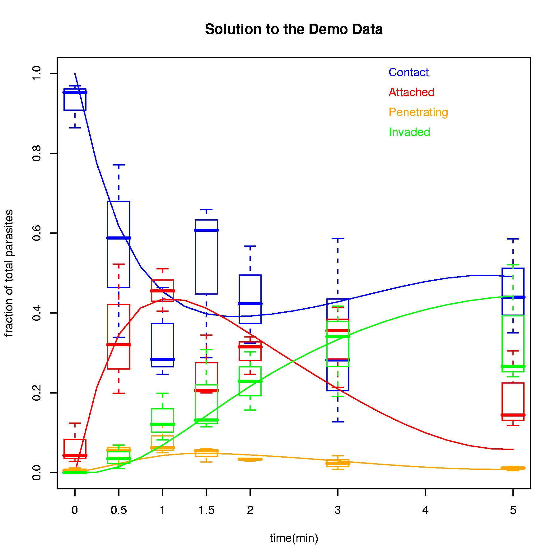
# Let's look at the fit with respect to the data
PlotModel(Demo$solution,Demo$sum,main="Solution to the Demo Data")

Sim<-NULL

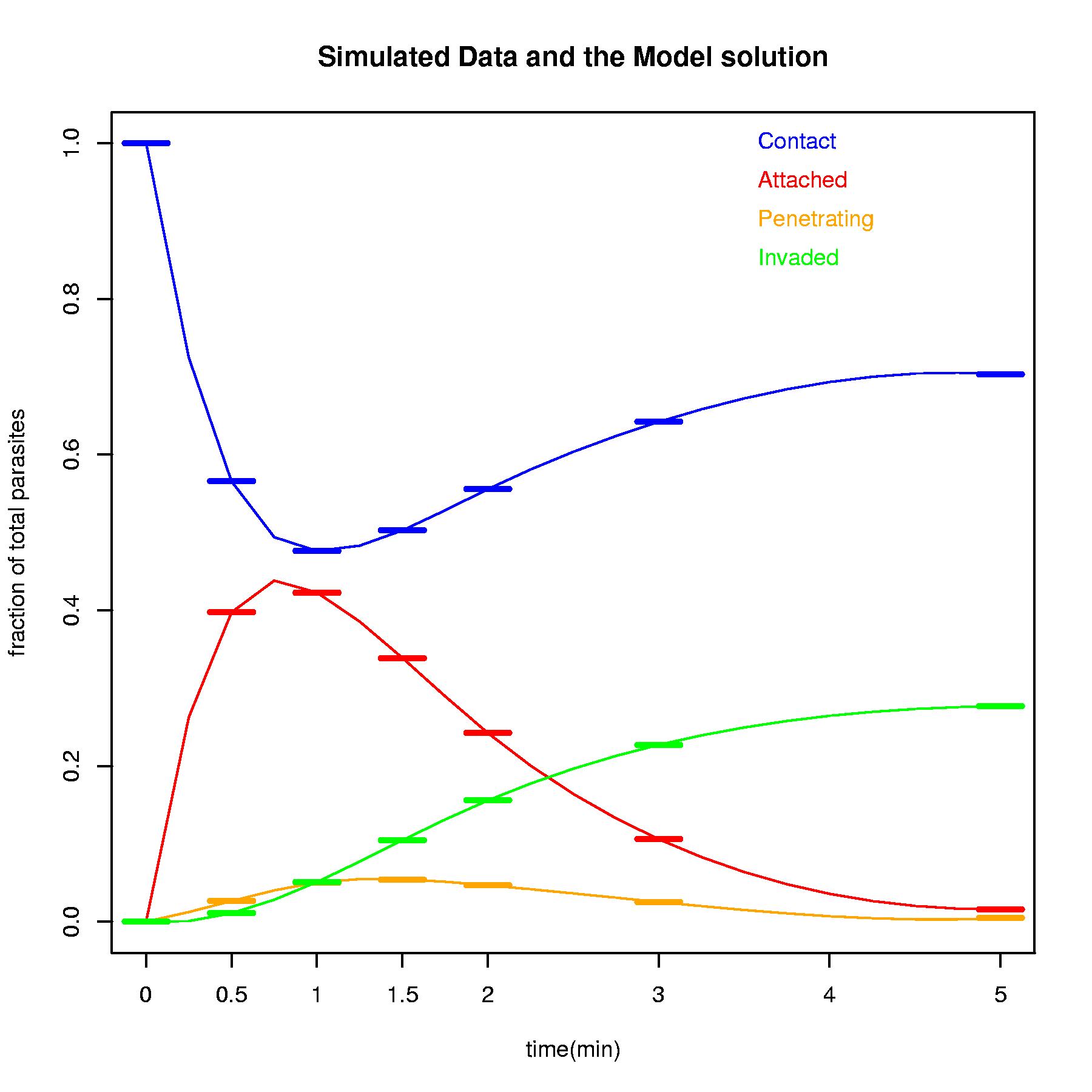
# We also can simulate some data given a Model and using a different set of parameters
Sim$sum<-SimData(5,Model,parms=c(1.5, 0.75, 0.3, 2.0))

# The model exactly find the original parameter and the fit looks perfect.
Sim$solution<-FitModel(Sim$sum,Model)

Sim$solution
$par
  k1   k2   k3   k4
1.50 0.75 0.30 2.00

$value
[1] 2.124532e-11

$counts
function gradient
      46       26

$convergence
[1] 0

$message
NULL

$init
[1] 1 0 0 0 0

$times
[1] 0.0 0.5 1.0 1.5 2.0 3.0 5.0

$model
function(t,y,p){       # System of ODEs describing the Model 
            yd1 <- - p[1] * y[1]
            yd2 <- + p[1] * y[1] - p[2] * y[2] - p[3] * y[2]
            yd3 <- + p[2] * y[2]
            yd4 <- + p[3] * y[2] - p[4] * y[4]
            yd5 <- + p[4] * y[4]
            list(c(yd1,yd2,yd3,yd4,yd5),c(massbalance=sum(y)))
}

$int.parms.guess
 k1  k2  k3  k4
1.0 1.0 0.5 3.0

$weights
[1] 1 1 5 1

$kinetics
  time       con          att          pen          inv sum
1  0.0 0.9999997 9.999996e-08 9.999996e-08 9.999996e-08   1
2  0.5 0.5655045 3.972677e-01 2.646774e-02 1.076007e-02   1
3  1.0 0.4761148 4.226993e-01 5.030598e-02 5.087992e-02   1
4  1.5 0.5024691 3.387022e-01 5.427147e-02 1.045573e-01   1
5  2.0 0.5554822 2.422344e-01 4.667966e-02 1.556038e-01   1
6  3.0 0.6418744 1.058099e-01 2.523780e-02 2.270779e-01   1
7  5.0 0.7032569 1.564765e-02 4.460424e-03 2.766350e-01   1

PlotModel(Sim$solution,Sim$sum,main="Simulated Data and the Model solution")