Motif Mapping

Tutorial 5: Motif Mapping

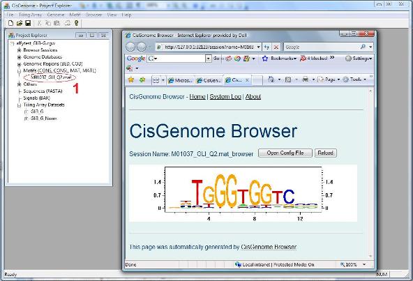
A dialog will jump out to let you choose the MAT file that contains your motif. After you add the file to the project, you should be able to see it in the Project Explorer Window, under the section “Motifs (CONS, CONSL, MAT, MATL)”. When you double click it (red circle 1 below), the sequence logo of the motif will be displayed in CisGenome Browser! (This is how you can visualize your motif using CisGenome Browser. Check the browser session file, I bet you will find more!).

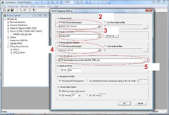
A dialog will show up. In this dialog, you need to specify:

1. A motif (i.e., a MAT file) (red circle 2 below);

2. A genome which the mapping will be based on (red circle 3);

3. A COD file that specifies input genomic regions where the motif will be mapped (red circle 4);

4. An output file that saves the result (red circle 5).

1. Motif Matrix Mapping

A motif can be represented by a matrix. To use CisGenome to map the matrix, the matrix needs to be stored in a text file in the following format (which we call MAT format):

1 1 1 100

1 10 90 1

1 5 95 1

1 1 100 1

10 1 1 90

1 1 100 1

5 5 90 1

6 1 1 100

1 100 1 1

Here, the four columns correspond to A, C, G, T respectively. Each row corresponds to a position in the motif. Each number in the matrix is a pseudo-count which is proportional to the relative frequency of the occurrence of a nucleotide at a given position. According to this definition, the sample motif above has a consensus pattern TGGGTGGTC.

To avoid log(0), before mapping the motif, CisGenome will automatically add a small positive number to each cell of the matrix. For this reason, we recommend you to use pseudo-count matrix instead of frequency matrix. In other words, in stead of using:

0.01 0.01 0.01 0.97

to represent relative frequency of A, C, G and T, it is much better to use

1 1 1 97

This will help alleviate the possible bias introduced by adding the small positive numbers.

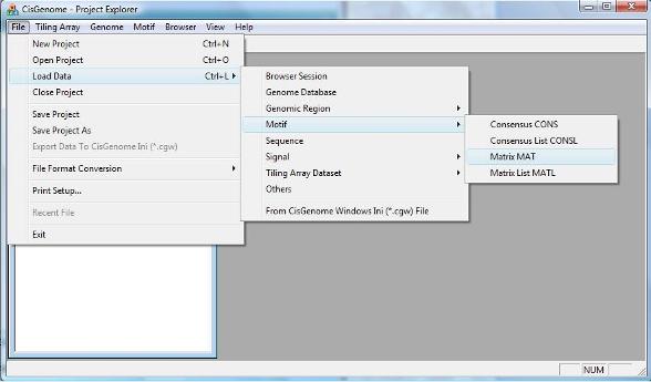
After you have prepared your motif matrix, you can load it to CisGenome by clicking the menu “File > Load Data > Motif > Matrix MAT”.

2. Motif Consensus Mapping

A second way to represent a motif is CONSENSUS sequence. In CisGenome, we use a text file in CONS format to store a CONSENSUS. Here is a sample CONS file:

TGGGT[A]GGTC[A,G,T]

In this example, the most frequent nucleotide at each position is TGGGTGGTC respectively. At position 5, T is allowed to be replaced by A; and at the last position, C is allowed to be replaced by A, G or T. For the motif here, we define TGGGTGGTC as the consensus, whereas TGGGT[A]GGTC[A,G,T] is defined as degenerate consensus. If a genomic sequence has the following pattern TGAGAGGTG, we say that the sequence has 3 mismatches to the consensus (MC=3) and 1 mismatch to the degenerate consensus (MD=1). When mapping a motif to genomes, you will be asked to set the maximal number of MC and the maximal number of MD allowed. All genomic loci that can satisfy your criteria will be reported as TFBS.

The procedure to perform consensus mapping is quite similar to matrix mapping. First, you need to use the menu “File > Load Data > Motif > Consensus CONS” to load the consensus to your project. Then you can click the menu “Motif > Known Motif Mapping > Single Consensus -> COD” or “Motif > Known Motif Mapping > Single Consensus -> FASTA”. A dialog will show up to guide you through the remaining procedure which is quite straightforward.

There are several public databases, including TRANSFAC and JASPAR, in which a large number of known transcription factor binding motifs are stored. Sometimes, the transcription factor you are studying may not have a known motif. What can you do? Don’t worry, there is a pretty good chance that you can recover it from your ChIP-chip binding data using de novo motif discovery which will be discussed now!

Using CisGenome, you can easily map a motif to the whole genome. For example, if you wish to map the motif to the mouse genome assembly mm8, you just need to find where mm8 database is installed. Within this folder, you can find a file named “chrlist.cod”. You can first add this file to your CisGenome Project using “File > Load Data > Genomic Region”, then you can using the motif mapping function described above to map the motif to chrlist.cod. As a result, you will get TFBS for the whole genome. In my PC, it usually take 30-60 min to run a whole genome mapping.

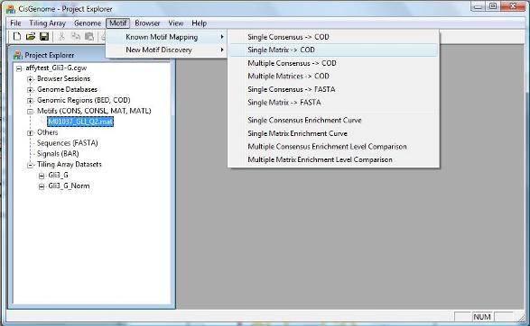
You can also map a motif matrix to a FASTA sequence file. In order to do so, click the menu “Motif > Known Motif Mapping > Single Matrix -> FASTA”. The usage is quite similar to what we have described above, please try it by yourself.

When you perform a ChIP-chip experiment, you are able to identify transcription factor binding regions at a 500bp resolution level. If you know the transcription factor binding motif, by mapping the motif to the binding regions, you may pinpoint individual transcription factor binding sites to a 6~30bp region. The high resolution binding site information will be extremely useful when you are trying to design knock-out animals. Mapping transcription factor binding motifs to genome sequences is also useful in many other contexts (e.g., computational prediction of important regulatory elements in co-regulated genes).

With CisGenome, transcription factor binding motif mapping becomes a fairly easy task. Both motif matrix and motif consensus can be mapped by CisGenome.

To map the motif to a collection of genomic regions, you can click the menu “Motif > Known Motif Mapping > Single Matrix -> COD”.

When the matrix is mapped to genome, at each location, it will be compared to a Markov Background Model. A location will be called a TFBS if the likelihood ration (LR) between the motif model and the Markov background model is bigger than a cutoff. By default, the cutoff is set to LR>=500. But you may change the cutoff to make it more stringent or less stringent.

You may also choose to use pre-computed Markov background models (which we recommend), or to use a background model estimated from input genomic regions.

As an optional parameter, you may choose to filter your TFBS by cross-species conservation, say, only keep TFBS that are located within 10% most conserved part of the genome, or only keep TFBS for which phastCons conservation score is greater than 40 (Note: phastCons scores range from 0 to 1, here we linearly scaled them to 0~255 to fit into one byte).

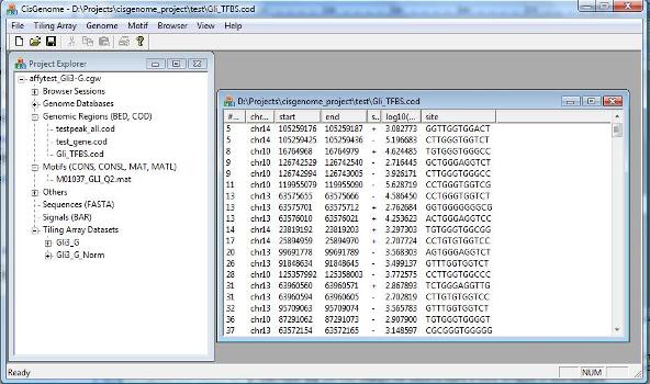
After you set all parameters, click “OK”. The program will start to run. After it finish, the results will be added to the Project Explorer window, under the section “Genomic Regions (BED, COD)”. A new window will also be opened to list all TFBS.