ChIP-seq Two Sample Analysis

Tutorial 2: ChIP-Seq Two Sample Analysis

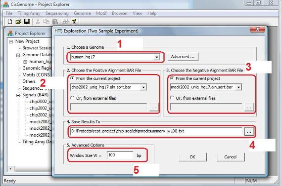
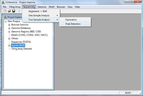
Similar to the one sample analysis, a two sample analysis starts with exploration. In this step, we will divide the genome into non-overlapping windows with fixed length W, and we will count how many IP reads (k1) and how many control reads (k2) are contained in each window. Conditional on the total window counts n=k1+k2, we will estimate the false positive rates for each (k1,k2) which will help us define the significance level.

To perform exploration, click the menu “Sequencing > Two Sample Analysis > Exploration”.

1. Exploration

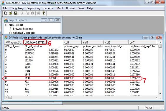
When the program finishes running, it will summarize model fitting results into a table (see below). Similar to the one sample analysis, the table reports how many windows (col2) have exactly n reads (col1, n=k1+k2), what percentage of windows (col3) have n reads, what is the expected percentage of windows that should have n reads under the poisson model (col4) and under the negative binomial model (col6), and the ratio between the expected percentage and the observed percentage under the two models (col5 and col7).

In addition to these numbers, there is a new number called “dP0_hat” (red circle 6). This is an important quantity that tells you, within a background window, what is the expected percentage of reads that will come from the IP sample (i.e., dP0_hat = E[k1/n]). dP0_hat will help us determine how big k1-k2 should be in order to call a window significant. Based on this number, false discovery rate for each (k1,k2) will be estimated, and the results will be saved to a file named “[outputfile_name].fdr”. Here [outputfile_name] is the name you gave in the red circle 4 above.

When we search for binding regions, windows with too few reads will not be considered. In our example here, a window with 8 reads corresponds to a false positive rate 6.96% under the negative binomial model (red circle 7), so we may choose to exclude windows with <8 reads in the peak detection step.

The step after exploration is peak detection. To detect binding regions in a two sample analysis, click the menu item “Sequencing > Two Sample Analysis > Peak Detection”.

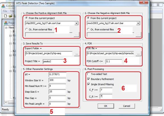
In the dialog that jumps out, you need to

1. choose the BAR file that contains the read-to-genome alignments for the IP sample (red circle 1);

2. choose the BAR file that contains the read-to-genome alignments for the control sample (red circle 2);

3. specify a working folder to store the output files and specify a project name for the analysis (red circle 3).

4. choose a FDR cutoff and the FDR file that contains pre-computed FDR for all (k1,k2) combinations (red circle 4). The FDR file is usually generated in the exploration step and has a filename “*.fdr”.

5. specify the expected fraction of IP reads in the background genomic regions (red circle 5), this is the dP0_hat obtained in the exploration step;

6. set window size W (red circle 5);

7. set the minimal read number cutoff C (red circle 5); windows with <C reads will be excluded from peak detection. In our example, we set the cutoff to be 8.

8. Optionally, you can also choose to perform post processing including boundary refinement and/or single strand filtering (red circle 6).

After you have set all the parameters, click “OK”, and the program will start to search for significant binding regions.

Note: CisGenome will produce a read density BAR file for visualization. To generate this file, a W bp sliding window with step size S will be used to scan the genome. When the “Step Size S” (in red circle 3) is small, you will need VERY BIG memory to be able to process the file. Very often, users don’t have sufficient memory, and as a result, nothing will be produced by CisGenome. You may think that something is wrong, but it is not. Indeed, if you set the Step Size S to a bigger number, for example, S = 100 bp instead of the default S = 25 bp, CisGenome will produce results for you.

A dialog will jump out. In the dialog, you need to

1. choose a genome (red circle 1);

2. choose a BAR file that contains the read-to-genome alignments for the ChIP sample (red circle 2);

3. choose a BAR file that contains the read-to-genome alignments for the control (Mock IP or Input) sample (red circle 3);

4. specify a file to save the model fitting results (red circle 4);

5. specify a window size W (red circle 5).

After you’ve set all the parameters, click “OK”.

2. Peak Detection

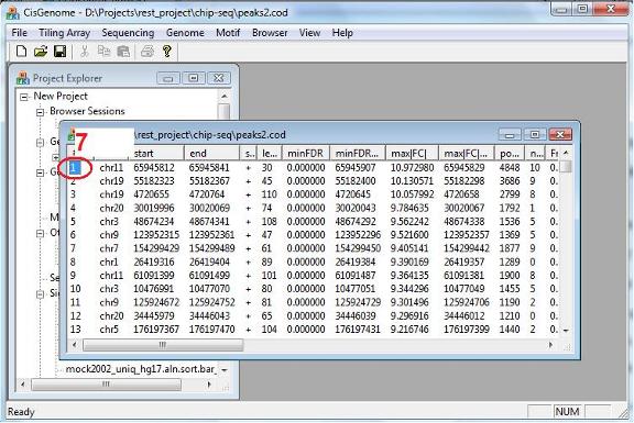
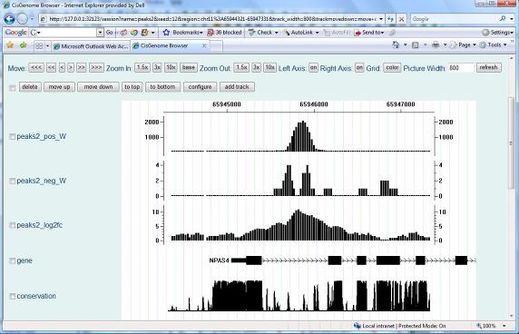
After the computation is done, a new window will show up to list all the peaks we found. You can again visualize the peaks by clicking the first column (circle 7) of the table.

When you reach this point, I would like to congratulate you since you have already learnt how to analyze a typical ChIP-seq experiment using CisGenome. Now take a break and relax a little bit before we learn more about CisGenome browser and data visualization!