
|
Tutorial 2: ChIP-Seq (SeqPeak) Data Analysis |
|
1.1 Download Genome Database Before you analyze the ChIP-seq data, you are strongly recommended to have necessary genome information stored in your local computer. Although this is not required by SeqPeak to call peaks from your data, the genome information can be helpful for visualization and for downstream analyses (e.g. motif discovery, associating peaks with genes). The genome information can be obtained from our download page which contains databases for various species. If you are studying mouse, for example, you can download the mouse genome database (e.g., mm8). This pre-compiled database contains all the necessary information required to support downstream visualization, annotation, sequence retrieval, and transcription factor binding motif mapping, etc. To download a genome database, simply click it and save it to a folder in your computer. The database usually has a “.gz”, “.zip” or “.exe” suffix. In the first two cases, after downloading you need to unzip the database using software such as gzip, unzip, WinZip, WinRAR etc. In the “.exe” case, the file is self-extractable, just double click it after downloading to install the database. The downloading procedure will take some time. While you are waiting, let’s continue our data preparation.
1.2 Prepare Alignment Files As the input of CisGenome, for each sample you’ve sequenced, you need to prepare a text file to provide the read-to-genome alignment information. The file should be tab-delimited and should have three columns as follows:
chr1[tab]359077[tab]F chr1[tab]376890[tab]R ….
This is called ALN format. A file in this format usually has a name ending with *.aln. In the file, column1 = chromosome where the read is aligned; column2 = coordinate where the read is aligned; column3 = ‘F’ or ‘+’: if the read is aligned to the forward strand of the genome assembly; ‘R’ or ‘-’: if the read is aligned to the reverse complement strand of the genome.
Many sequencing platforms produce alignment information as their output. For example, data generated by Illumina/Solexa are usually aligned using ELAND algorithm. If you use these alignments, please convert them to the ALN format before CisGenome analysis. If your alignment is generated by ELAND, you can convert it to the ALN format by using the menu “File > File Format Conversion > ELAND->ALN”. If your alignment is generated by bowtie, you can convert it to the ALN format by using the menu “File > File Format Conversion > Bowtie->ALN”. If your alignment is in BED format, you can convert it to the ALN format by using the menu “File > File Format Conversion > Bed->ALN”. Please make sure that the genome database downloaded from CisGenome website is consistent with the genome assembly used for read alignment. After you have downloaded the genome database and prepared the input ALN files, you are ready to move on to the next step -- peak calling. Here is an example data set with ALN files for you to play with peak calling (unzip it before using; use human hg18 genome). |
1. Data Preparation |
|
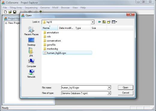
A dialog will jump out to ask you to select a genome database. Go to the folder where you have installed/unzipped your database. Within the database folder, you should be able to find a file with a “.cgw” suffix. Usually this file is named as “[species]_[version].cgw”, e.g., human_hg18.cgw. Choose this file, and click the “Open” button. |
|
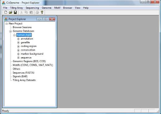
If the database is loaded correctly, you should be able to see a new item in the Project Explorer Window now, under “Genome Databases” (as shown below). |
2. Peak Calling |
|
When you start CisGenome, it automatically opens an empty data analysis project. If you have downloaded the genome database from our website, you can load it into CisGenome before peak calling (although this is not required).
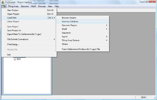
2.1 Loading Genome Database (Optional) To load a genome database, click the menu “ File > Load Data > Genome Database” . |
|
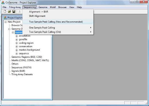
2.2 Peak Calling You can now call peaks by clicking the menu “Sequencing > Two Sample Peak Calling (New and Recommended)”. |
|
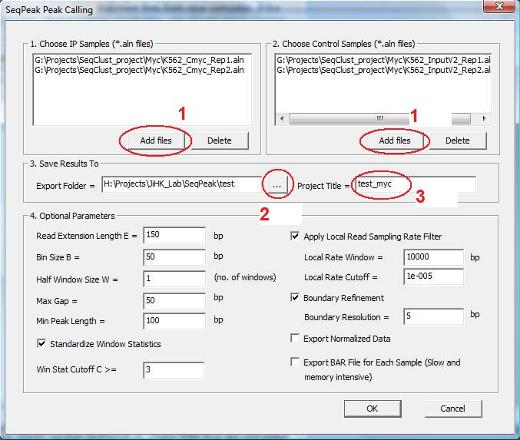
A dialog will jump out. In the dialog, first click the button “Add files” (highlighted by the red circle 1) to choose IP and control samples. After you click the button, an “Open” file dialog will appear to allow you to add one or more alignment (*.aln) files to the project. You can use the “Delete” button to remove the files you don’t want to analyze. |
|
Next, click the button highlighted by red circle 2 to choose a folder to export your analysis results. In the project title box (red circle 3), provide a name for the project. There are a number of optional parameters you can set. These include: (1) Read Extension Length E: reads with be extended E base pairs to 3’ ends. The extended DNA fragments will be used to determine genome coverage. (2) Bin Size B: the genome will be divided into non-overlapping bins, each B bp long. For each bin, the program will count how many DNA fragments cover the bin. Later, the counts will be normalized across samples, taking into account of sequencing depths, and the normalized counts will be used to call peaks. (3) Half Window Size W: To determine enrichment signal, each bin and its 2*W flanking bins (W on the left and W on the right) will be combined into a window. The normalized DNA fragment counts in these 2*W+1 bins will be compared between IP and control samples. A t-statistic similar to the TileMap t-statistic (formula 6 in the paper) will be computed. The t-statistic will be used as the window statistic for the center bin. For transcription factors (narrow peaks), the value of W is usually chosen such that (2W+1)*B = 150 ~ 500. For histone modifications (broad peaks), the value of W is usually chosen such that (2W+1)*B = 500 ~1000. Note: CisGenomev1 uses a conditional binomial model to determine enrichment. Our internal tests show that the t-statistic method and the conditional binomial method perform similarly well in non-replicate data. However, since the t-statistic method can be used to analyze replicate data and takes into account cross-sample variability whereas the binomial method cannot, CisGenomev2 adopts the t-statistic approach to measure signal enrichment. (4) Standardize Window Statistics: If checked, the window statistics across all bins will be standardized by subtracting genome-wide mean and dividing by genome-wide standard deviation. (5) Win Stat Cutoff C >=: Bins with window statistic >= C will be called as peaks. Peak false discovery rate (FDR) will be determined by flipping IP and control labels. The FDR will be reported in the output file. Therefore, SeqPeak does not use FDR as a parameter for peak calling. However, users can use the FDR reported in the results to further filter peaks. (6) Apply Local Read Sampling Rate Filter / Local Rate Window / Local Rate Cutoff: This is the MACS type of filter. It uses control reads in 10 kb (or X bp specified by “Local Rate Window”) flanking windows of a bin to estimate a local read sampling rate R. The total number of ChIP reads in the bin is compared to a Poisson distribution with rate R. If the p-value is bigger than “Local Rate Cutoff”, then the bin will be excluded from peak calling even if its window statistic might be bigger than the cutoff C. Empirically, this filter is useful for filtering out bins close to repeat regions but having low read counts. (7) Max Gap: If the distance between two peaks are smaller than Max_Gap bp, then they will be merged into one peak. (8) Min Peak Length: If the peak length is smaller than Min_Peak_Length bp, then the peak will not be reported. (9) Boundary Refinement / Boundary Refinement Resolution: After peaks are detected, we use a finer bin (5 bp by default or Y bp specified by “Boundary Refinement Resolution”) to analyze forward and reverse strand reads separately. The offset between the forward and reverse strand peaks will be used to determine the refined peak boundaries. This is very useful for narrowing down the transcription factor binding sites to a resolution of <50 bp. (10) Export Normalized Data: If checked, the normalized DNA fragment counts will be reported for each sample and each peak. (11) Export BAR File for Each Sample: If checked, the bin read counts for each sample will be exported and saved to BAR files. BAR files can be visualized in CisGenome browser. This step requires lots of memory and computation time. (The old version of CisGenome often breaks down here). If not checked, the program will still export two bar files for visualization (a BAR file for window statistic, and a BAR file for log2 fold enrichment between normalized IP and control read counts), but it will take much less memory and computation time.
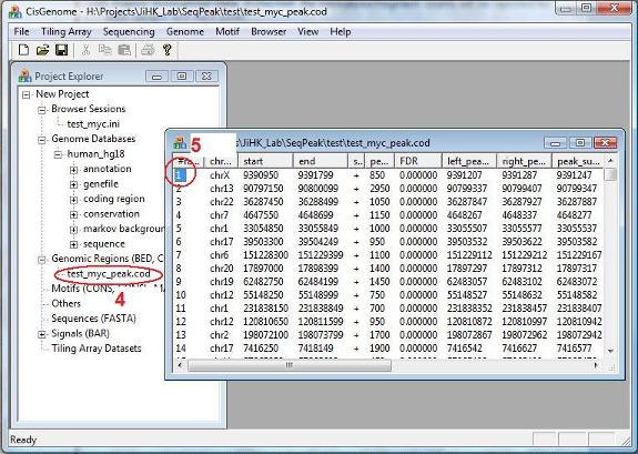
After you have set all the parameters, click the “OK” button. Now the program will start to work. After the computation is done, you will see a new item in the Project Explorer, under the “Genomic Regions (BED, COD)”. The item has the name you specified, and has an extension “_peak.cod” (red circle 4). This is a tab-delimited text file that contains the detected peaks. When you double click the item, a new window will show up which lists all the detected peaks. (Note: in the current version of CisGenome, this window will automatically jump out after peak detection).
|
|
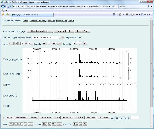
Now try to choose a peak, and click the first column (the red circle 5). Have you seen anything?. |
|
If you see the above “CisGenome Browser” window jumping out in your Internet Explorer, congratulations, you have successfully performed peak detection from your ChIP-seq data! Now you can visually check data quality for each individual peak, simply by clicking the peak in your peak list. CisGenome browser is a powerful tool for visualizing the genomic signals. We will introduce more about it shortly. But before that, let’s first discuss two things Next> |