Tutorial 2: ChIP-Seq One Sample Analysis

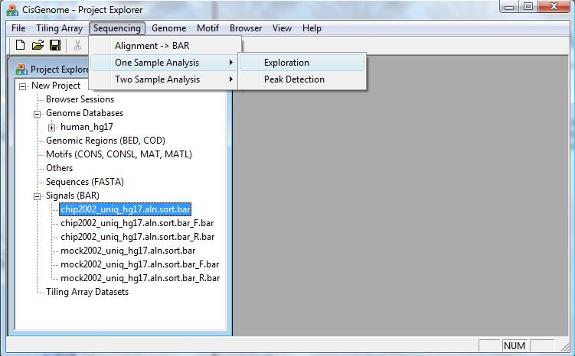
Before a genome-wide search for binding signals, we need to understand statistical properties of the genomic distribution of the millions of sequence reads. This is a step we call “exploration”, in which we will fit a parametric model to describe the count of reads in a fixed-length window. More precisely, we will divide the genome into non-overlapping windows with fixed length W, and we will count how many window have exactly 0 read, 1 read, 2 reads, 3 reads, and so on. We will fit this distribution with a poisson and a negative binomial model. By comparing the observed number of windows that have k reads with the expected number of windows that have k reads, we can estimate the false positive rate, which will then tell us how many reads a window should have in order to become significant. 

To perform exploration, click the menu “Sequencing > One Sample Analysis > Exploration”.

1. Exploration

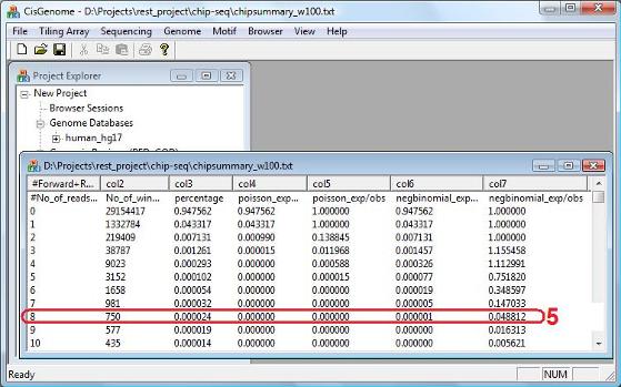
The model fitting results will be summarized in a table (see below). From the table, you will know how many windows (col2) have exactly k reads (col1), and what percentage of windows (col3) have k reads. The table will also tell you what is the expected percentage of windows that should have k reads under the poisson model (col4) and under the negative binomial model (col6). The ratio between the expected percentage and the observed percentage gives you an estimated false positive rate (col5 and col7).

In the example shown here, the negative binomial model provides a better fit of the data. Under this model, a window with 8 reads will have a false positive rate 4.88% (red circle 5).

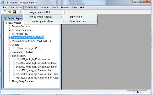
The model fitting results provide the basis for detecting binding regions (or peaks). To detect peaks, click the menu “Sequencing > One Sample Analysis > Peak Detection”.

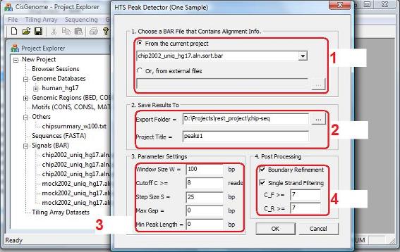
In the dialog that jumps out, you need to choose the BAR file that contains the read-to-genome alignments (red circle 1). You also need to specify a working folder to store the analysis results, and give a common title to name the output files (red circle 2). In the “Parameter Settings” section (red circle 3), you can set window size W, significance cutoff C, as well as a few other parameters. For example, if we want to control the false positive rate <= 10%, we can set the cutoff to be 8 which, according to the exploration results, has a false positive rate 4.88% under the negative binomial model. Optionally, you can also choose to perform post processing including boundary refinement and/or single strand filtering. After you have set all the parameters, click “OK”, and the program will start to search for significant binding regions.

Note: CisGenome will produce a read density BAR file for visualization. To generate this file, a W bp sliding window with step size S will be used to scan the genome. When the “Step Size S” (in red circle 3) is small, you will need VERY BIG memory to be able to process the file. Very often, users don’t have sufficient memory, and as a result, nothing will be produced by CisGenome. You may think that something is wrong, but it is not. Indeed, if you set the Step Size S to a bigger number, for example, S = 100 bp instead of the default S = 25 bp, CisGenome will produce results for you.

 

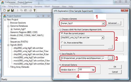
Now a dialog will jump out. In the dialog, first choose a genome (red circle 1), then choose a BAR file that contains the read-to-genome alignments for the ChIP sample you have (red circle 2). Next, click the button “…” and specify a file to save the model fitting results (red circle 3), and specify a window size W (red circle 4). After you’ve done all these, click “OK”. The program will start to run.

2. Peak Detection

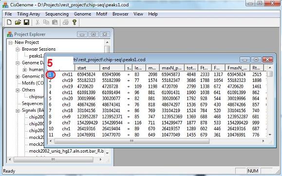
After the computation is done, you will see a new item in the Project Explorer, under the “Genomic Regions (BED, COD)”. The item has the name you’ve given, and has an extension “.cod”. This is indeed a tab-delimited text file that contains peaks you’ve detected.

When you double click the item, a new window will show up, in which all the peaks are listed. (Note: in the new version of CisGenome, this window will automatically jump out after peak detection).

Now try to choose a peak, and click the first column (the red circle 5). Have you seen anything?

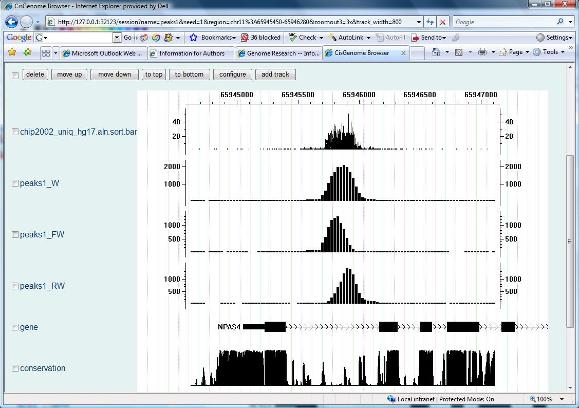
If you see the following “CisGenome Browser” window jumping out in your Internet Explorer, congratulations, you have now reached the most exciting part of data analysis! You can now visualize your sequencing data! You can  visually check data qualities for each individual peak, simply by clicking the peak in your peak list.

There are a lot of things you can do with the CisGenome browser. Before we formally introduce the browser, however, let’s first continue our lessons on ChIP-seq data analysis and learn how to handle a typical two sample experiment in which both a ChIP sample and a control sample have been sequenced. Next>