
|
Tutorial 2: Tiling Array Analysis (cont.) |
|
Since you have already created a tiling array data set, you can start to analyze it. However, before we do that, you need to know two important techniques, i.e. how to save your project and how to open a project. They are important because you can then save your project at any time, and next time you want to revisit your project, you don’t need to repeat all the analyses you’ve already done.
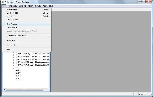
To save you current project, click menu “File > Save Project”. A dialog will show up to help you save your project to a CisGenome Windows Project (*.cgw, or CGW) file.
|
2. Save and open your project |
|
After you saved your project, you can try to close your project by clicking “File > Close Project”.
You can then try to reload your project by choosing the menu “File > Open Project”. Once again, a dialog will jump out and ask you to choose a CGW file to open. After you open the file, you will be able to see all the data in the project in the CisGenome Project Explorer Window.
Remember to save your project frequently to avoid loss of your analysis efforts. |
3. Data Normalization |
|
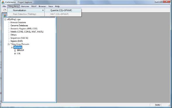
Before we try to search for peaks (e.g. protein-DNA binding regions in a ChIP-chip experiment), we need to first normalize the array data to remove systematic bias. To normalize your tiling array data, click menu “Tiling Array > Normalization > Quantile (CEL+BPMAP)”. (Let’s try quantile first. MAT normalization will be incorporated soon). |
|
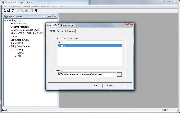
A dialog will show up. You need to specify which data set to analysis, and where to save your results.
Note: There is another page called “Advanced (Optional)” in the dialog which will allow advanced users to set up normalization parameters. For the tutorial here, we don’t need to worry about it.
Now you can click OK on the bottom of the dialog. The normalization program will start to run.
|
|
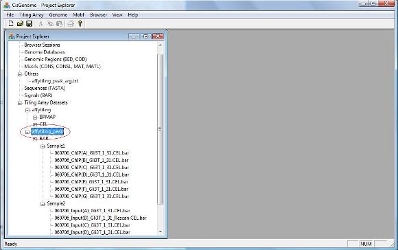
After normalization has been done, you will be able to see a new item added to the CisGenome Project Explorer Window (the tree view window), under the Tiling Array Datasets. Now you are ready to search for real signals! |
4. Peak Detection |
|
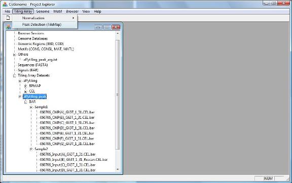
To find peaks from your data, click menu “Tiling Array > Peak Detection (TileMap)”. |
|
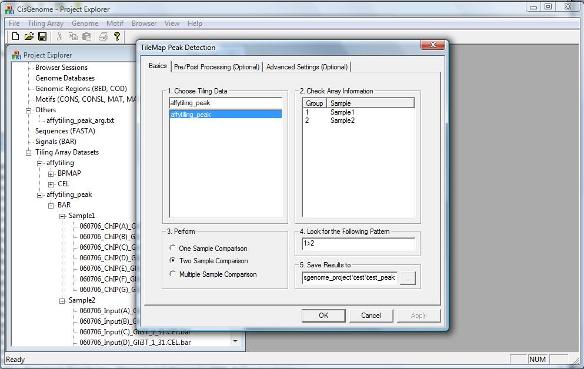
A dialog will jump out. You need to 1. choose a normalized tiling array data set to analyze; 2. specify what types of analysis (one sample, two sample or multiple sample comparisons) will be performed; 3. tell the computer what is the pattern you are looking for (e.g., 1>2. Remember when we created the data, 1=IP, 2=Input, 1>2 here means IP>Input, i.e. ChIP-chip binding regions). 4. specify a file to save the results. Again, there are two other optional pages for advanced users. We don’t need to worry about them in the tutorial here. Click “OK”, and the program will start to run!
|
|
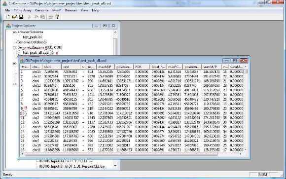
After the computation is done, you will see a new item in the Project Explorer, under the “Genomic Regions (BED, COD)” (see the red circle A below). The item has the name you’ve given, and has an extension “_all.cod”. This is indeed a tab-delimited text file that contains peaks you’ve detected. When you double click the item, a new window will show up, in which all the peaks are listed. (Note: in the new version of CisGenome, this window will automatically jump out after peak detection). Now try to choose a peak, and click the first column (the red circle B). Have you seen anything? |
|
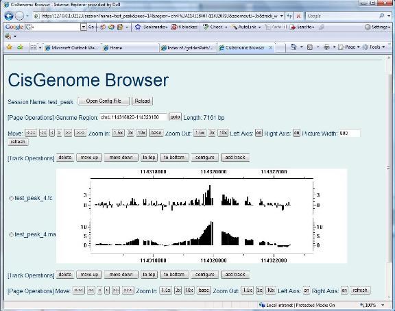
If you see the following “CisGenome Browser” window jumping out in your Internet Explorer, congratulations, you have now reached the most exciting part of data analysis! You can now visualize your tiling array data! You are now able to visually check data qualities for each individual peak, simply by clicking the peak in your peak list. |
|
Now let’s take a break, reward yourself with some cookies before we go to the next section: visualization! |