
|
Tutorial 3: Visualizing Gene Annotations |
|
When you start this page, you should have downloaded your genome database. If the database you downloaded ends with “.gz” or “.zip”, you need to unzip it using gzip, unzip, WinZip, WinRAR or other software. If the database you downloaded ends with “.exe”, you just need to double click it to install, since this is a self-extractable file.
With the genome database available, you can now add gene annotations to your track. You can either add them automatically or you can add them manually.
|
|
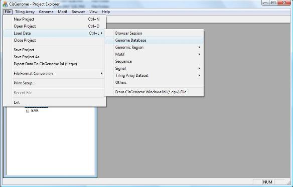
A dialog will jump out to ask you select a genome database. Go to the folder where you installed/unzipped your database. Within the database folder, you should be able to find a file with a “.cgw” suffix. Usually this file is named as “[species]_[version].cgw”, e.g., mouse_mm8.cgw. Choose this file, and click “Open” button. |
|
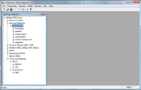
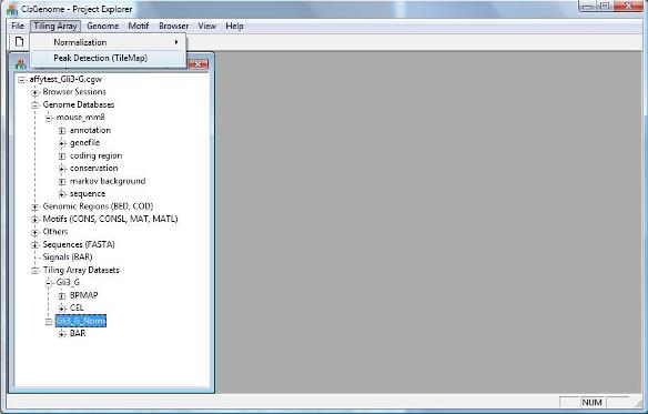
If the database is loaded correctly, you should now see a new item in the Project Explorer Window, under “Genome Databases” (as shown below). |
|
Now you can rerun tiling array peak detection by clicking the menu “Tiling Array > Peak Detection (TileMap)”. In case you forget how to run it, please revisit the tiling array analysis tutorial. |
|
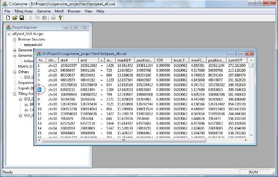
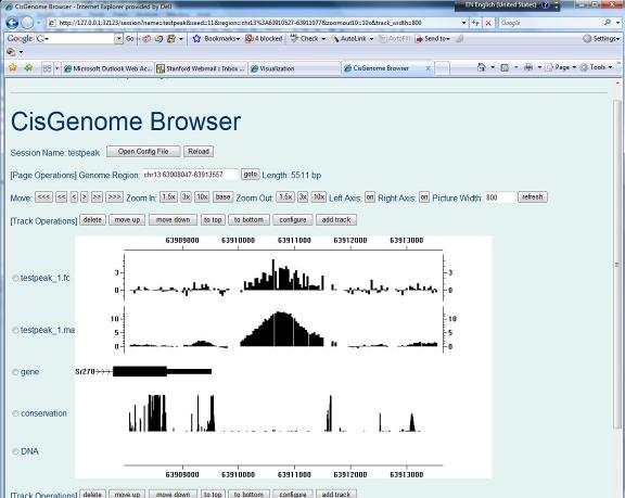
After you run peak detection, a list of peaks will be reported. Randomly choose one and click on its first column. What do you see? If nothing wrong, you should now have a CisGenome Browser session in which tiling array signals are displayed side-by-side with gene structures, cross-species conservation and DNA sequences! |
1. Add Gene Annotations Automatically |
|
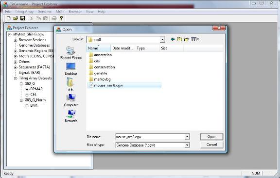
In order to add gene annotations automatically to your display, you need to rerun your tiling array peak detection. First, let’s go back to the CisGenome GUI and add the genome database to our project. To add a genome database, click menu “ File > Load Data > Genome Database” . |
2. Add Gene Annotations Manually |
|
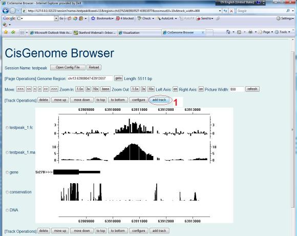
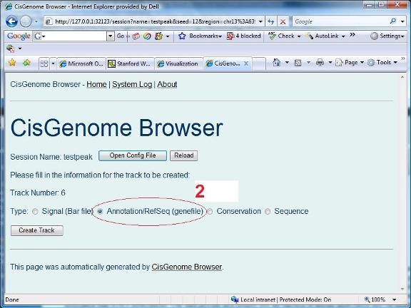
To add gene annotations manually to your browser session, first click “add track” button (red circle 1) on your browser page. |
|
A new page will show up to let you choose the track type. Let’s first choose “Annotation/RefSeq(genefile)” (red circle 2). |
|
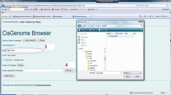
Another page will show up. In this page, first specify a name for the track (red circle 3), and then choose a annotation file by clicking “Browse...” (red circle 4). The gene structure annotation can be found from where your genome database is installed. For example, if your database is located at D:\genomes\mouse\mm8\, then you should choose D:\genomes\mouse\mm8\genefile\mm8.genefile. |
|
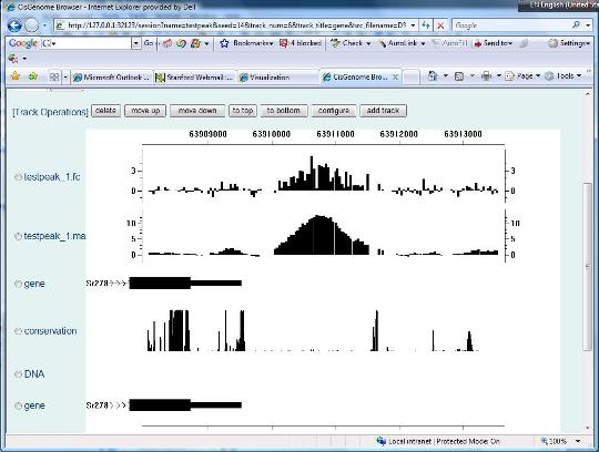
After you click the “Update Track” button, your session page will be updated, and a new track that shows gene structures will be added.
You can follow similar steps to add DNA sequences and conservation scores manually. For example, to add sequences, you can choose track type = sequence, and using folder D:\genomes\mouse\mm8\. To add conservation scores, set track type = conservation, and folder = D:\genomes\mouse\mm8\conservation\phastcons\ |
|
At this point, you’ve already learnt a lot about CisGenome Browser. However, until now it was mainly used to visualize genomic regions. Indeed, the CisGenome Browser can also be used to visualize raw array images and motif sequence logos. The visualization of raw array images has already been explained in session 2: tiling array analysis, and we will explain how to visualize motif sequence logo’s in session 5: motif analysis. Since you’ve already learnt one of the most important functions of CisGenome, it’s time for you to take a break, reward yourself with some drinks and cookies. After the break, we will move on to the exciting sequence and motif analysis! Next >> |