Peter Murakami: power and sample size

getpower(), getpower.mlm(), and getpower.mlm.ri() functions

added July 22, 2010

Code File

The code for the getpower, getpower.mlm, and getpower.mlm.ri functions is contained in the file getpower.R. You can source the file directly into R by calling

      source("http://www.biostat.jhsph.edu/~pmurakam/getpower.R")

The code is licensed under the GNU General Public License version 3, or (at your option) any later version.

Manual page

Description:
Power calculations for many analyses are difficult, not implemented, limited, and/or non-existent
in closed form. These functions calculate power for many different types of analysis through simulation.
These functions offer the ability to investigate power and sample size when any number of study design
characteristics are altered.
By calculating power for various different sample size alternatives, the right sample size for your power
of choice can be found.

- getpower returns power for simple linear regression, simple logistic regression, and simple poisson
regression.
- getpower.mlm.ri returns power for simple linear regression, simple logistic regression, and simple
poisson regression, with a random intercept.
- getpower.mlm returns power for linear regression, logistic regression, and poisson regression, with
a random intercept and random coefficient, and fixed effects for treatment and time. See chapter 20
in Data Analysis Using Regression and Multilevel/Hierarchical Models by Gelman/Hill for fuller
explanation.

Note that getpower.mlm.ri can also be used to get power for GEE gaussian model with uniform correlation
structures, since a gaussian marginal model with uniform correlation structure is equivalent to a gaussian
model with just a random intercept.

Usage:
getpower(n, n.sim=1000, covariate, b1, b0=0, alpha=.05, getps=FALSE, fam, sigma.y, Offset=rep(0,n), ...)

getpower.mlm(J, K, n.sims=1000, fam="gaussian", mu.a.true, g.0.true,g.1.true, sigma.y.true, sigma.a.true,
sigma.b.true, Offset=rep(0,J*K), rho=0, ...)

getpower.mlm.ri(J, K, n.sims=1000, fam="gaussian", covariate, B1, mu.a.true, sigma.a.true, sigma.y.true,
Offset=rep(0,J*K), ...)

Arguments for getpower:
n - sample size.
n.sim - number of iterations to run.
alpha - the significance level at which you reject the null hypothesis.
fam - "gaussian","binomial", or "poisson", indicating the distribution of the outcome data.
"binomial" will be analyzed by logistic regression with logit link, and "poisson" will be
analyzed by poisson regression with log link.
b0 - true value of beta_0. Values that are not extreme make the random samples that get
generated more representative. E.g., if we're only taking a sample of 30 and lambda in the rpois
is .005, the resulting sample will not be too good. Also, in logistic regression for example,
setting b0 determines what probabiilities the desired OR corresponds to. E.g., if you want to
detect an OR difference of 1.25 that corresponds to p0=.05 and p1=.062, set b1=log(1.25) and b0=-2.995.
b1 - smallest value of b1 you want to be able detect.
getps - tells whether you want the function to return all the n p-values for b1 (getps=TRUE) or just the
power (getps=FALSE). Set to true for, e.g., function diagnostic purposes.
sigma.y - true standard deviation of the outcome. Specify this if fam="gaussian".
Offset - if given, for fam="poisson", must already by logged, since that's what glm takes.
covariate - the values of the covariate. It can be a numeric or integer vector of length n (e.g., rep(c(0,1),n/2)),
or an expression for obtaining a random sample (e.g., expression(rnorm(n,0,2)) or
expression(rpois(n,3))).

Arguments for getpower.mlm:
J - number of subjects
K - number of measurements/subject
n.sim - number of iterations to run.
fam - can be "gaussian","binomial", or "poisson". Link functions will be the canonical ones.
mu.a.true - true average value of random intercept, the true link(outcome) at t=0
g.0.true - true average slope for the controls
g.1.true - smallest true average effect, at each time, of the treatment that you want to be able
to detect, except time=0 since treatment doesn't affect the slope in this model since this
model assumes treatment can have no effect at time=0.
sigma.y.true - true sd of the outcome. Needed if outcome is gaussian.
sigma.a.true - true sd of the random intercept.
sigma.b.true - true sd of the random coefficient.
rho - the true correlation between intercepts and slopes. 0 (independence, since they're gaussian)
by default.
Offsets must already be logged, as in glm().

Arguments for getpower.mlm.ri:
J - number of clusters
K - number of measurements/cluster
n.sim - number of iterations to run.
fam - can be "gaussian","binomial", or "poisson". Link functions will be the canonical ones.
mu.a.true - true average value of random intercept, the true link(outcome) at t=0
sigma.a.true - true sd of the random intercept.
covariate - numeric or integer vector of length K, or an expression for obtaining a random sample of size J*K.
sigma.y.true - true sd of the outcome. Needed if outcome is gaussian.
B1 - smallest value of b1 you want to be able detect.
Offsets must already be logged, as in glm().

NOTE:
1. alpha is assumed to be .05 for getpower.mlm and getpower.mlm.ri.
2. Power calculations based on simple (only 1 predictor variable) regression models (like
the above functions assume) also apply to multiple regression settings if the additional q
covariates added (which should be thought to be correlated with the outcome) are uncorrelated
with the covariate of interest (i.e., if they are added to improve precision rather than
because they are confounders) and the expected increase in precision (i.e., decrease in the
standard deviation of the error term) exactly offsets the effect of reducing the number of
degrees of freedom. If the expected increase in precision gained by adding the extra q
covariates exceeds the effect of losing q degrees of freedom, the power returned will
be too low (and sample sizes obtained will be larger than needed). If the expected increase
in precision does not equal or exceed the effect of losing q degrees of freedom, the power
returned will be too high (and sample sizes obtained will be smaller than needed), however in
that case you would probably not want to include these additional covariates in the first
place.

This is demonstrated in the formula for the estimate of the standard error of the estimate of b
in the model Y = a + bX + U:

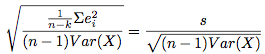
compared to the formula for the estimate of the standard error of the estimate of b in the 
model Y = a + bX + cZ + U:

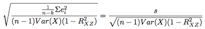
In these equations, U is the random error term, e are residuals, i indexes the observations 
from 1 to n, k is the number of parameters that are being estimated, and R denotes correlation. 
All errors are assumed to be uncorrelated with one another.  n-k decreases as we add more 
covariates, however on the other hand, the additional covariates may lead to a decrease in the 
sum of squared residuals (increased precision).  I think the same ideas apply to 
non-OLS models as well, however i do not have a proof of this.

See Also:
GLIMMPSE
The longpower package in R
The clusterPower package in R
The optimalAllocation package in R
See Stata's stpower command for cox proportional hazards models.


EXAMPLES FOR GETPOWER:

#Checks:
pp = getpower(n.sim=2000,n=300,b1=0,fam="poisson",covariate=rep(c(.2,.5,1),100),getps=TRUE)
binom.test(mean(pp<=.05)*2000,2000,p=.05) #Not significant.  Good.  CI includes .05.
hist(pp) #uniform.  good.  more uniform the larger the sample size is.  With few observations, the 
#normal approximation doesn't hold as well, so the coefficient will not be as close to normally distributed.

#Example of poisson model with offset:
getpower(n=60,n.sim=500,b1=0,fam="poisson",covariate=rep(c(.2,.5,1.0),20),Offset=log(rnorm(60,20,5)))

#Example of logistic regression:
#This result was verified by PASS sample size software:
getpower(n=4160,n.sim=1000,b1=log(1.25),b0=-2.995,fam="binomial",
         covariate=rep(c(0,1),c(round(.84*4160),round(.16*4160))))

#A test: make sure the function returns approximately the known power of the t-test, since the 2-sample 
#t-test of equal means (equal variances) is equivalent to SLR:
power.t.test(n=100,delta=3,sd=10)
getpower(n=200,n.sim=3000,b1=3,fam="gaussian",covariate=rep(c(0,1),100),sigma.y=10) #It does. Good.

#Get sample size for various powers:
powers = vector("numeric",length=8)
k=1
for(i in seq(from=10,to=80,by=10)){
    powers[k] = getpower(n=i*3, n.sim=1000,b1=.65,fam="poisson",covariate=rep(c(.2,.5,1.0),i))
    k=k+1
}
plot(powers~seq(from=10,to=80,b=10),type="l",ylab="Power",xlab="sample size per level")

#Example where independent variable values are unknown beforehand:
#Say the independent variable of interest is some gaussian rv (centered around 0).
getpower(n=25,n.sim=2000,b1=2,covariate=expression(rnorm(25,0,5)),fam="gaussian",sigma.y=15)


EXAMPLES FOR GETPOWER.MLM:

#Examples, using few iterations for speed.  In practice should do more.
getpower.mlm(J=120, K=7, n.sims=200, mu.a.true=4.8, g.0.true= -.5, g.1.true=.5, sigma.a.true=1.3, 
             sigma.b.true=.7, fam="gaussian", sigma.y.true=.7,rho=.1)

#Check.  This should be around .05, but is usually lower.  Not certain why it's conservative, but
#it is probably because the approximation to the correct reference t-distribution used is imperfect--
#how many degrees of freedom to use is still an unsettled question (see "The trouble with 
#calculating p-values for estimates from mixed effects models" on the Links page).  
#The same thing happens when using the code from the book, with no changes at all.
getpower.mlm(J=120, K=15, n.sims=200, mu.a.true=4.8, g.0.true= -.5, g.1.true=0, sigma.a.true=1.3, 
             sigma.b.true=.7, fam="gaussian", sigma.y.true=.7,rho=.1) 

#Example of poisson model:
getpower.mlm(J=120, K=7, n.sims=50, mu.a.true=.5, g.0.true= -.5, g.1.true=.5, sigma.a.true=2, 
             sigma.b.true=1,fam="poisson",rho=.1)

#Example of logistic model:
getpower.mlm(J=120, K=7, n.sims=50, mu.a.true=.4, g.0.true= -.5, g.1.true=.5, sigma.a.true=1, 
             sigma.b.true=.4,fam="binomial",rho=.1)

#Get power for various sample sizes:
for(i in c(120,130,140)) print(getpower.mlm(J=i, K=7, n.sims=500, mu.a.true=4.8, g.0.true= -.5, 
                                            g.1.true=.5, sigma.y.true=.7, sigma.a.true=1.3, 
                                            sigma.b.true=.7,rho=0)) 


EXAMPLES FOR GETPOWER.MLM.RI:

#Examples, using few iterations for speed.  In practice should do more.
#Sometimes models with random data will be unfittable and warning messages will be printed. It's OK.
getpower.mlm.ri(J=100, K=3, n.sims=200, covariate=1:3, fam="gaussian", B1=0, mu.a.true=5, 
                sigma.a.true=2, sigma.y.true=6)

getpower.mlm.ri(J=50, K=7, n.sims=500, covariate=expression(rnorm(350,0,6)), fam="gaussian", B1=0, 
                mu.a.true=5, sigma.a.true=1, sigma.y.true=1)

getpower.mlm.ri(J=30, K=3, n.sims=300, covariate=0:2, fam="poisson", B1=log(1.2), mu.a.true=-1, sigma.a.true=2)

getpower.mlm.ri(J=30, K=3, n.sims=300, covariate=0:2, fam="poisson", B1=log(1.2), mu.a.true=-1, sigma.a.true=2, 
                Offset=log(sample(1:10,size=90,replace=TRUE)))

getpower.mlm.ri(J=120, K=7, n.sims=100, covariate=1:7, fam="binomial", B1=log(1.5), mu.a.true=4, sigma.a.true=1)

pw = vector()
k=1
for(i in c(60,70,80)) {
    pw[k] = getpower.mlm.ri(J=i, K=3, n.sims=500, covariate=1:3, fam="gaussian", B1=1, mu.a.true=5, 
                            sigma.a.true=2, sigma.y.true=4)
    k=k+1
}
pw